We could fit a model with the survival package:
library(survival)## Loading required package: splinessurv_fit <- survfit(coxph(Surv(time, status) ~ age + sex, lung))
surv_fit## Call: survfit(formula = coxph(Surv(time, status) ~ age + sex, lung))
##
## records n.max n.start events median 0.95LCL 0.95UCL
## 228 228 228 165 320 285 363Tidying this object lets us create a survival curve with ggplot2:
library(broom)
td <- tidy(surv_fit)
head(td)
## time n.risk n.event n.censor estimate std.error conf.high conf.low
## 1 5 228 1 0 0.9958207 0.004189316 1.0000000 0.9876776
## 2 11 227 3 0 0.9832688 0.008446584 0.9996823 0.9671247
## 3 12 224 1 0 0.9790670 0.009474977 0.9974188 0.9610529
## 4 13 223 2 0 0.9706383 0.011286679 0.9923495 0.9494021
## 5 15 221 1 0 0.9664127 0.012106494 0.9896182 0.9437513
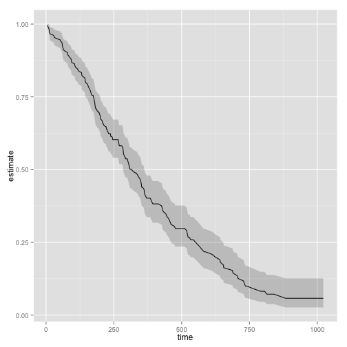
## 6 26 220 1 0 0.9621802 0.012883740 0.9867862 0.9381877library(ggplot2)
ggplot(td, aes(time, estimate)) + geom_line() +
geom_ribbon(aes(ymin = conf.low, ymax = conf.high), alpha = .2)